COS4852 Assignment 1¶

UNISA SCHOOL OF COMPUTING COS4852 SOFTWARE ENGINEERING

Assignment number: 1 Submission date: 29/04/2024 Name: Clifton Bartholomew Student number: 58362525

title: "## Table of Contents"

QUESTION 1:¶

A First Encounter - Link: https://citeseerx.ist.psu.edu/document?repid=rep1&type=pdf&doi=6ba8ead7ab2f7d1fd40ccf4381b662b8c6ed3c07 - Size: 417 KB

An introduction to machine learning: - Link: http://ai.stanford.edu/~nilsson/MLBOOK.pdf - Size:1855 KB

NOTE TO MARKER: Apologies, I ran out of time and could not complete Q2,3,6.

QUESTION 2:¶

(INCOMPLETE) Research

Read Nilsson’s book, Chapter 2. Summarise the chapter in 2-4 pages in such a way that you can show that you thoroughly understand the concepts described there. Use different example functions from the ones in the book to show that you understand the concepts

DNF -> Decision lists Decision Lists Partitioning space (linear separability) - using DNF. DNF -> binary decision trees.

Representation
- Boolean algebra
- Diagrammatic representations
Classes of Boolean Functions
- Terms and Clauses
- DNF Functions
- CNF Functions
- Decision Lists
- Symmetric and Voting Functions
- Linearly Separable Functions

QUESTION 3:¶

(INCOMPLETE) Research

Chapter 5 of Welling’s book Write a short research report (2-4 pages) that describes the k-Nearest Neighbours (kNN) algorithm and its variants. Your report must show a complete kNN algorithm as well as a detailed, worked example with all the steps and calculations. Use the following data set in your worked example:

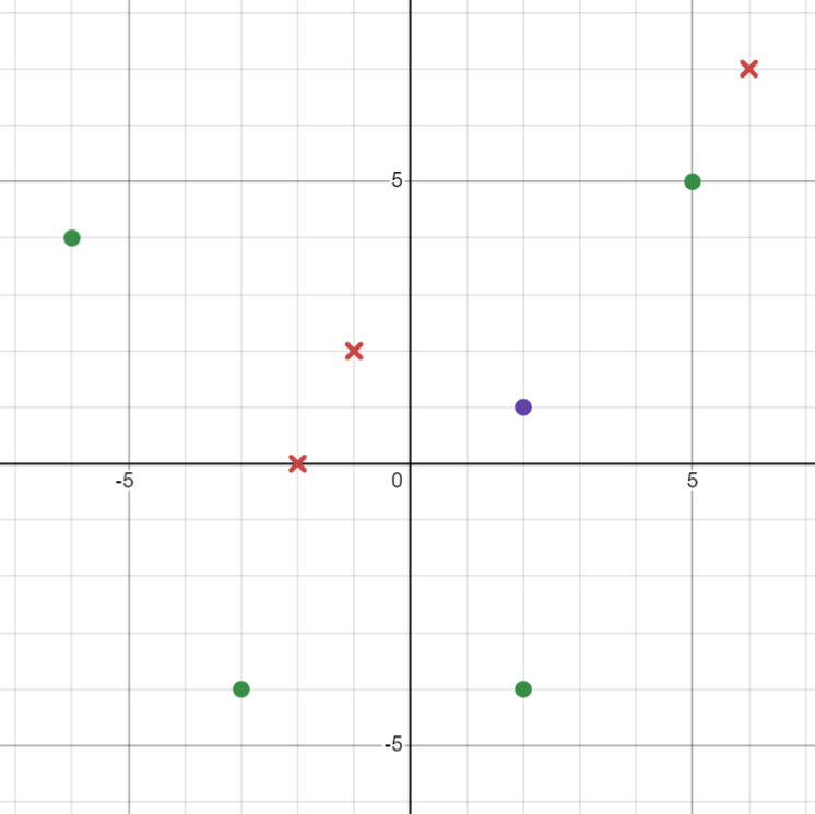
Positive instances: $$ \begin{align} \ P_1 &= (5,5,P)\ P_2 &= (-6,4,P)\ P_3 &= (-3,-4,P)\ P_4 &= (2,-4,P)\ \end{align} $$

Negative instances: $$ \begin{align} \ N_1 &= (-1,2,N)\ N_2 &= (-2,0,N)\ N_3 &= (6,7,N)\ N_4 &= (8,-8,N)\ \end{align} $$

Pasted image 20240429212751.png { width="400" }

Classify $Q_{1} = (2, 1, c)$ using the kNN algorithm.

Using the Euclidian distance measure: $$ d_{Euclidian}(p,q) = \sqrt{(p_x-q_x)^2+(p_y-q_y)2} $$

The distance between $Q_{1}$ and the other 8 instances with their ranks according to the closest distance is as follows:

Pasted image 20240429225140.png

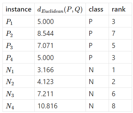
Using $k = \sqrt{n}$ we get a $k$ value of $2.82$ or $3$ .

With $k = 3$ , the 3 closest neighbours gives 2 tied positive instances and 2 negative instances. Thus we would not be able to classify $Q_{1}$ as positive or negative.

With $k = 2$ , we would classify $Q_{1}$ as negative.

With $k = 4$ , we would not be able to classify $Q_{1}$ (same reasoning as $k = 3$ ).

With $k = 5$ , we would classify $Q_{1}$ as positive.

QUESTION 4:¶

This problem is centered on Concept Learning. Can we use the given set of labelled training data to find a hypothesis/hypotheses that can correctly classify new data points being added to the version space.

In order to answer this question we must: 1. Create a set of all hypotheses that fit the version space. 2. Define a measure that can identify which of two hypotheses is more general or more specific that the other. i.e. find a suitable more_general_than relation. 3. Use that measure to order the hypotheses in the set from most specific to most general.

Assumptions¶

Based on the input data given, assume values of $a$ and $b$ be restricted to: $0 < a <= 10$ and $0 < b <= 10$
Assume that we are only considering the donut hypotheses (no other shapes).

Tools¶

Desmos | Graphing Calculator LaTeX - A document preparation system

Create set of all hypotheses that fit version space¶

With the assumptions made above, if $H$ has the form $h \leftarrow ⟨ a < \sqrt{x^{2} + y^{2}} < b ⟩$ where $a < b$ and $a, b \in Z$ ( $Z$ only contains non-negative integers, ${0, 1, 2, 3, . . .}$ ) and this can be shortened to $h \leftarrow ⟨ a, b ⟩$ then the set $H$ of all the hypotheses will consist of the following elements:

\begin{aligned} H = { & ⟨ 0, 1 ⟩, ⟨ 0, 2 ⟩, ⟨ 0, 3 ⟩, ⟨ 0, 4 ⟩, ⟨ 0, 5 ⟩, \\ ⟨ 0, 6 ⟩, ⟨ 0, 7 ⟩, ⟨ 0, 8 ⟩, ⟨ 0, 9 ⟩, ⟨ 0, 10 ⟩, \\ ⟨ 1, 2 ⟩, ⟨ 1, 3 ⟩, ⟨ 1, 4 ⟩, ⟨ 1, 5 ⟩, ⟨ 1, 6 ⟩, \\ ⟨ 1, 7 ⟩, ⟨ 1, 8 ⟩, ⟨ 1, 9 ⟩, ⟨ 1, 10 ⟩, ⟨ 2, 3 ⟩, \\ ⟨ 2, 4 ⟩, ⟨ 2, 5 ⟩, ⟨ 2, 6 ⟩, ⟨ 2, 7 ⟩, ⟨ 2, 8 ⟩, \\ ⟨ 2, 9 ⟩, ⟨ 2, 10 ⟩, ⟨ 3, 4 ⟩, ⟨ 3, 5 ⟩, ⟨ 3, 6 ⟩, \\ ⟨ 3, 7 ⟩, ⟨ 3, 8 ⟩, ⟨ 3, 9 ⟩, ⟨ 3, 10 ⟩, ⟨ 4, 5 ⟩, \\ ⟨ 4, 6 ⟩, ⟨ 4, 7 ⟩, ⟨ 4, 8 ⟩, ⟨ 4, 9 ⟩, ⟨ 4, 10 ⟩, \\ ⟨ 5, 6 ⟩, ⟨ 5, 7 ⟩, ⟨ 5, 8 ⟩, ⟨ 5, 9 ⟩, ⟨ 5, 10 ⟩, \\ ⟨ 6, 7 ⟩, ⟨ 6, 8 ⟩, ⟨ 6, 9 ⟩, ⟨ 6, 10 ⟩, ⟨ 7, 8 ⟩, \\ ⟨ 7, 9 ⟩, ⟨ 7, 10 ⟩, ⟨ 8, 9 ⟩, ⟨ 8, 10 ⟩, ⟨ 9, 10 ⟩} \end{aligned}

Define a generalization/specificity measure¶

For a given hypothesis, $h$ , to be valid it must include all the positive instances and exclude all the negative instances. - A maximally general hypothesis includes as much of the version space as possible without including any negative instances. - A maximally specific hypothesis includes as little of the version space without excluding any of the positive instances.

Since we are talk about "taking up space", a natural generality measure would be to use area of the donut hypothesis as indicated below: $$ \begin{align} h\langle a,b \rangle & : A = \pi (a^2 - b^2) \end{align} $$

This would give an area for each of hypothesis as follows: $$ \begin{align} h\langle 0,1 \rangle & : A = \pi ( 1^2-02 ) = \pi \ h\langle 0,2 \rangle & : A = \pi ( 2^2-02 ) = 4\pi \ h\langle 0,3 \rangle & : A = \pi ( 3^2-02 ) = 9\pi \ h\langle 0,4 \rangle & : A = \pi ( 4^2-02 ) = 16\pi \ h\langle 0,5 \rangle & : A = \pi ( 5^2-02 ) = 25\pi \ h\langle 0,6 \rangle & : A = \pi ( 6^2-02 ) = 36\pi \ h\langle 0,7 \rangle & : A = \pi ( 7^2-02 ) = 49\pi \ h\langle 0,8 \rangle & : A = \pi ( 8^2-02 ) = 64\pi \ h\langle 0,9 \rangle & : A = \pi ( 9^2-02 ) = 81\pi \ h\langle 0,10 \rangle & : A = \pi ( 10^2-02 ) = 100\pi \ h\langle 1,2 \rangle & : A = \pi ( 2^2-12 ) = 3\pi \ h\langle 1,3 \rangle & : A = \pi ( 3^2-12 ) = 8\pi \ h\langle 1,4 \rangle & : A = \pi ( 4^2-12 ) = 15\pi \ h\langle 1,5 \rangle & : A = \pi ( 5^2-12 ) = 24\pi \ h\langle 1,6 \rangle & : A = \pi ( 6^2-12 ) = 35\pi \ h\langle 1,7 \rangle & : A = \pi ( 7^2-12 ) = 48\pi \ h\langle 1,8 \rangle & : A = \pi ( 8^2-12 ) = 63\pi \ h\langle 1,9 \rangle & : A = \pi ( 9^2-12 ) = 80\pi \ h\langle 1,10 \rangle & : A = \pi ( 10^2-12 ) = 99\pi \ h\langle 2,3 \rangle & : A = \pi ( 3^2-22 ) = 5\pi \ h\langle 2,4 \rangle & : A = \pi ( 4^2-22 ) = 12\pi \ h\langle 2,5 \rangle & : A = \pi ( 5^2-22 ) = 21\pi \ h\langle 2,6 \rangle & : A = \pi ( 6^2-22 ) = 32\pi \ h\langle 2,7 \rangle & : A = \pi ( 7^2-22 ) = 45\pi \ h\langle 2,8 \rangle & : A = \pi ( 8^2-22 ) = 60\pi \ h\langle 2,9 \rangle & : A = \pi ( 9^2-22 ) = 77\pi \ h\langle 2,10 \rangle & : A = \pi ( 10^2-22 ) = 96\pi \ h\langle 3,4 \rangle & : A = \pi ( 4^2-32 ) = 7\pi \ h\langle 3,5 \rangle & : A = \pi ( 5^2-32 ) = 16\pi \ h\langle 3,6 \rangle & : A = \pi ( 6^2-32 ) = 27\pi \ h\langle 3,7 \rangle & : A = \pi ( 7^2-32 ) = 40\pi \ h\langle 3,8 \rangle & : A = \pi ( 8^2-32 ) = 55\pi \ h\langle 3,9 \rangle & : A = \pi ( 9^2-32 ) = 72\pi \ h\langle 3,10 \rangle & : A = \pi ( 10^2-32 ) = 91\pi \ h\langle 4,5 \rangle & : A = \pi ( 5^2-42 ) = 9\pi \ h\langle 4,6 \rangle & : A = \pi ( 6^2-42 ) = 20\pi \ h\langle 4,7 \rangle & : A = \pi ( 7^2-42 ) = 37\pi \ h\langle 4,8 \rangle & : A = \pi ( 8^2-42 ) = 48\pi \ h\langle 4,9 \rangle & : A = \pi ( 9^2-42 ) = 65\pi \ h\langle 4,10 \rangle & : A = \pi ( 10^2-42 ) = 84\pi \ h\langle 5,6 \rangle & : A = \pi ( 6^2-52 ) = 11\pi \ h\langle 5,7 \rangle & : A = \pi ( 7^2-52 ) = 24\pi \ h\langle 5,8 \rangle & : A = \pi ( 8^2-52 ) = 39\pi \ h\langle 5,9 \rangle & : A = \pi ( 9^2-52 ) = 56\pi \ h\langle 5,10 \rangle & : A = \pi ( 10^2-52 ) = 75\pi \ h\langle 6,7 \rangle & : A = \pi ( 7^2-62 ) = 13\pi \ h\langle 6,8 \rangle & : A = \pi ( 8^2-62 ) = 28\pi \ h\langle 6,9 \rangle & : A = \pi ( 9^2-62 ) = 45\pi \ h\langle 6,10 \rangle & : A = \pi ( 10^2-62 ) = 64\pi \ h\langle 7,8 \rangle & : A = \pi ( 8^2-72 ) = 15\pi \ h\langle 7,9 \rangle & : A = \pi ( 9^2-72 ) = 32\pi \ h\langle 7,10 \rangle & : A = \pi ( 10^2-72 ) = 51\pi \ h\langle 8,9 \rangle & : A = \pi ( 9^2-82 ) = 17\pi \ h\langle 8,10 \rangle & : A = \pi ( 10^2-82 ) = 36\pi \ h\langle 9,10 \rangle & : A = \pi ( 10^2-92 ) = 19\pi \ \end{align} $$

Order the list from most specific to most general¶

Sorted from most specific to most general this list becomes: $$ \begin{align} h\langle 0,1 \rangle & : A = \pi \ h\langle 1,2 \rangle & : A = 3\pi \ h\langle 0,2 \rangle & : A = 4\pi \ h\langle 2,3 \rangle & : A = 5\pi \ h\langle 3,4 \rangle & : A = 7\pi \ h\langle 1,3 \rangle & : A = 8\pi \ h\langle 0,3 \rangle & : A = 9\pi \ h\langle 4,5 \rangle & : A = 9\pi \ h\langle 5,6 \rangle & : A = 11\pi \ h\langle 2,4 \rangle & : A = 12\pi \ h\langle 6,7 \rangle & : A = 13\pi \ h\langle 1,4 \rangle & : A = 15\pi \ h\langle 7,8 \rangle & : A = 15\pi \ h\langle 0,4 \rangle & : A = 16\pi \ h\langle 3,5 \rangle & : A = 16\pi \ h\langle 8,9 \rangle & : A = 17\pi \ h\langle 9,10 \rangle & : A = 19\pi \ h\langle 4,6 \rangle & : A = 20\pi \ h\langle 2,5 \rangle & : A = 21\pi \ h\langle 5,7 \rangle & : A = 24\pi \ h\langle 1,5 \rangle & : A = 24\pi \ h\langle 0,5 \rangle & : A = 25\pi \ h\langle 3,6 \rangle & : A = 27\pi \ h\langle 6,8 \rangle & : A = 28\pi \ h\langle 2,6 \rangle & : A = 32\pi \ h\langle 7,9 \rangle & : A = 32\pi \ h\langle 1,6 \rangle & : A = 35\pi \ h\langle 0,6 \rangle & : A = 36\pi \ h\langle 8,10 \rangle & : A = 36\pi \ h\langle 4,7 \rangle & : A = 37\pi \ h\langle 5,8 \rangle & : A = 39\pi \ h\langle 3,7 \rangle & : A = 40\pi \ h\langle 2,7 \rangle & : A = 45\pi \ h\langle 6,9 \rangle & : A = 45\pi \ h\langle 1,7 \rangle & : A = 48\pi \ h\langle 4,8 \rangle & : A = 48\pi \ h\langle 0,7 \rangle & : A = 49\pi \ h\langle 7,10 \rangle & : A = 51\pi \ h\langle 3,8 \rangle & : A = 55\pi \ h\langle 5,9 \rangle & : A = 56\pi \ h\langle 2,8 \rangle & : A = 60\pi \ h\langle 1,8 \rangle & : A = 63\pi \ h\langle 0,8 \rangle & : A = 64\pi \ h\langle 6,10 \rangle & : A = 64\pi \ h\langle 4,9 \rangle & : A = 65\pi \ h\langle 3,9 \rangle & : A = 72\pi \ h\langle 5,10 \rangle & : A = 75\pi \ h\langle 2,9 \rangle & : A = 77\pi \ h\langle 1,9 \rangle & : A = 80\pi \ h\langle 0,9 \rangle & : A = 81\pi \ h\langle 4,10 \rangle & : A = 84\pi \ h\langle 3,10 \rangle & : A = 91\pi \ h\langle 2,10 \rangle & : A = 96\pi \ h\langle 1,10 \rangle & : A = 99\pi \ h\langle 0,10 \rangle & : A = 100\pi \ \end{align} $$

Question 4(a) S-Boundary Set¶

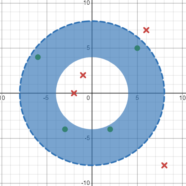
The four positive instances are $(5, 5)$ , $(- 6, 4)$ , $(- 3, - 4)$ and $(2, - 4)$ .

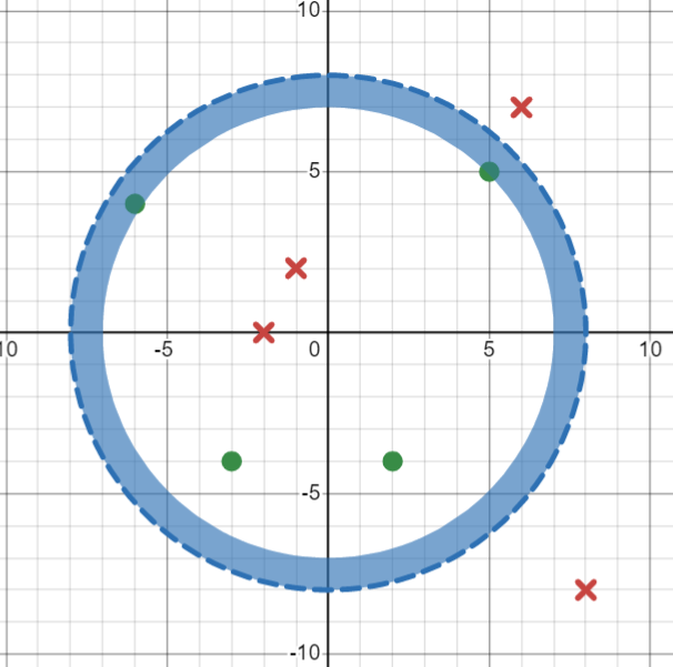
If we consider the instance $(5, 5)$ the most specific hypothesis to include this point is: $h \leftarrow ⟨ 7, 8 ⟩$

Pasted image 20240423205636.png { width="400" }

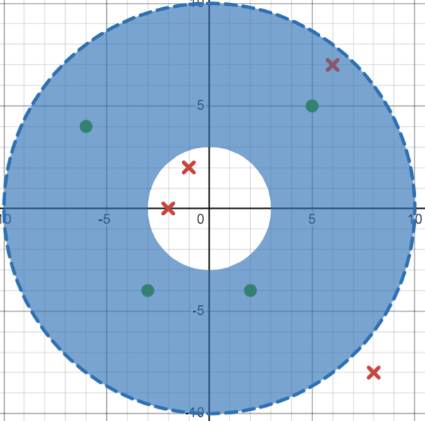
If we consider the final positive instance $(- 6, 4)$ , this is already included in the current hypothesis and this the hypothesis does not change.

If we consider the next positive instance $(- 3, - 4)$ , we must expand the hypothesis to $h \leftarrow ⟨ 4, 8 ⟩$ to include this instance:

Pasted image 20240423210341.png { width="400" }

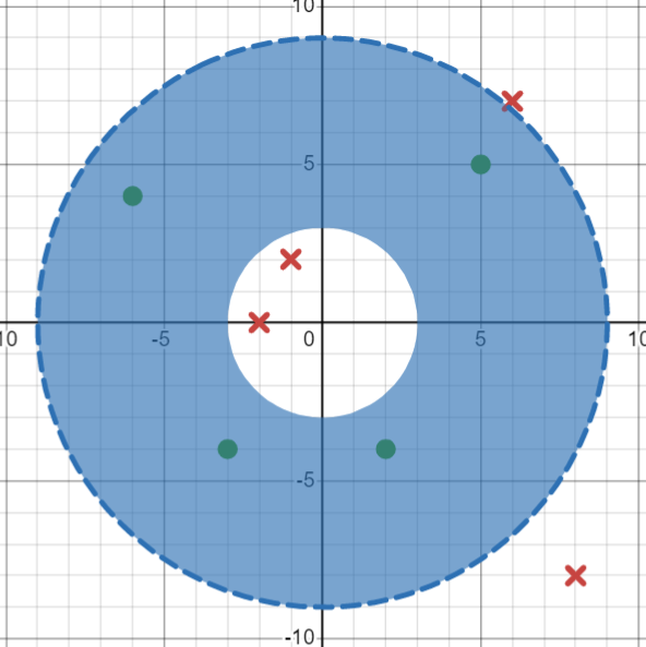
If we consider the final positive instance $(2, - 4)$ , this is already included in the current hypothesis and this the hypothesis does not change.

This gives a final S-boundary set of $S = {⟨ 4, 8 ⟩}$

Question 4b) G-Boundary Set¶

The four negative instances are $(- 1, 2)$ , $(- 2, 0)$ , $(6, 7)$ and $(8, - 8)$ .

If we consider the instance $(- 1, 2)$ the most general hypothesis to exclude this instance is: $h \leftarrow ⟨ 3, 10 ⟩$

Pasted image 20240423212044.png { width="400" }

This hypothesis also excludes instances $(- 2, 0)$ and $(8, - 8)$ so the hypothesis does not need to change.

To exclude instance $(6, 7)$ , we must contract the hypothesis to $h \leftarrow ⟨ 3, 9 ⟩$ Pasted image 20240423212449.png { width="400" }

This gives a final G-boundary set of $G = {⟨ 3, 9 ⟩}$

Question 4(c) New Data¶

A new positive instance $p = (6, - 6)$ would increase the S-boundary set to $S = {⟨ 4, 9 ⟩}$ .

A new negative instance $q = (6, 6)$ would decrease the G-boundary set to $S = {⟨ 3, 8 ⟩}$ .

Question 4(d) Alternative hypothesis space¶

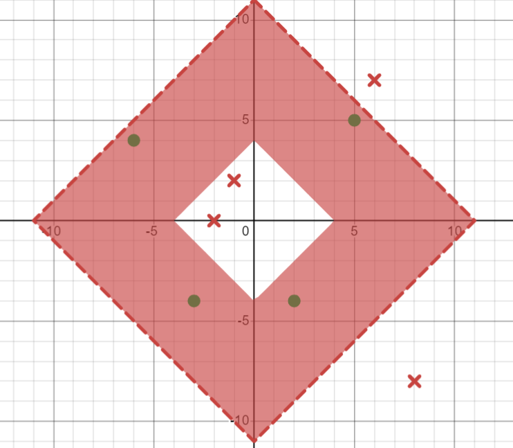
Consider the set of diamond donut hypotheses $H$ which has the form form $h \leftarrow ⟨ a < | x | + | y | < b ⟩$ where $a < b$ and $a, b \in Z$ ( $Z$ only contains non-negative integers, ${0, 1, 2, 3, . . .}$ )

$h \leftarrow ⟨ 4, 11 ⟩$ will be an instance which separates the given data as shown below: Pasted image 20240423232926.png { width="400" }

QUESTION 5:¶

I did not draw out the full binary decision trees and then try and simplify them, rather I analysed the output of the boolean function to look for patterns and construct the tree from there. My explanations of my thought process are placed before each of the binary decision trees.

Tools¶

Flowchart Maker & Online Diagram Software

Question 5(a)¶

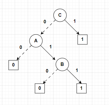
Consider the truth table for the function $f_{1} (A, B, C) = C \lor (A \land B)$

Pasted image 20240429225318.png

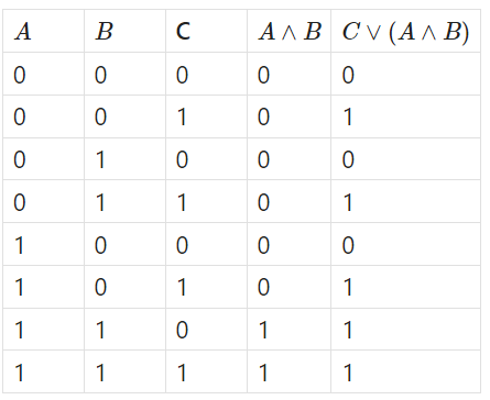
I chose $C$ as the root since a true value for $C$ will always result in a true value for the whole function. If $C$ is false, then both $A$ and $B$ must be true in order to reach the true leaf, otherwise it will lead to a false leaf.

The binary decision tree will be as follows: Pasted image 20240424000304.png

Question 5(b)¶

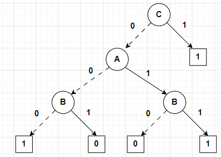
Consider the truth table for the function $f_{1} (A, B, C) = (A \lor B) \Rightarrow C$

Pasted image 20240429225347.png

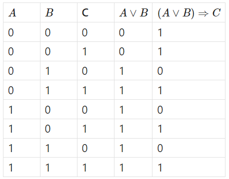
I chose $C$ as the root again since the implication is true whenever $C$ is true. When $C$ is false, the only two decision paths that will result in true are when $A$ and $B$ are both false or both true.

The binary decision tree will be as follows: Pasted image 20240424123558.png

Question 5(c)¶

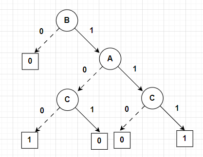
Consider the truth table for the function $f_{3} (A, B, C) = B \land (A \Leftrightarrow C)$

Pasted image 20240429225423.png

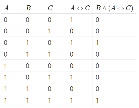
In this question I chose $B$ as the root since it is the limiting variable (whenever $B$ is false, the whole function is false). When $B$ is true, the only paths that lead to true are when $A$ and $C$ are both true or both false.

The binary decision tree will be as follows: Pasted image 20240424201135.png

Question 5(d)¶

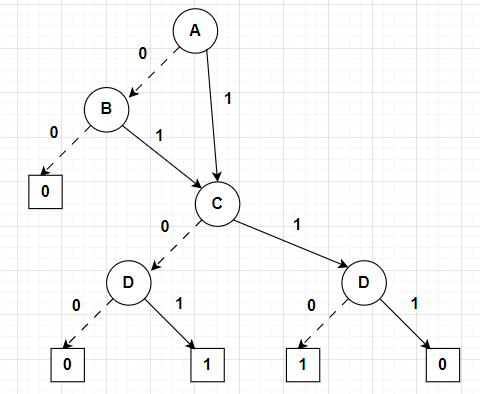
Consider the truth table for the function $f_{4} (A, B, C, D) = (A \lor B) \land (C ⊻ D)$

Pasted image 20240429225447.png

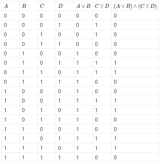
Since the function is almost similar to the $C ⊻ D$ and is only limited by whether $A$ and $B$ are both false. I started with $A$ and $B$ and terminated the decision tree if both were false, then went into the $C ⊻ D$ portion of the binary decision tree.

The binary decision tree will be as follows: Pasted image 20240424204443.png

QUESTION 6¶

(INCOMPLETE)

This question is based on the ID3 algorithm used to construct binary decision trees.

Node Search: Root Node¶

#	TimeOfDay	EnergyLevel	PreviousAttendance	AssignmentDue	Attend?
1	Morning	High	Yes	Yes	Yes
2	Evening	Low	No	Yes	No
3	Evening	High	Yes	No	Yes
4	Afternoon	Medium	Yes	Yes	Yes
5	Morning	Low	No	No	No
6	Afternoon	Low	No	Yes	No
7	Evening	Medium	No	No	Yes
8	Afternoon	Low	Yes	Yes	No
9	Morning	High	Yes	No	Yes
10	Evening	Low	Yes	Yes	Yes
11	Afternoon	High	No	No	Yes
12	Morning	Medium	Yes	Yes	No
13	Afternoon	High	Yes	No	Yes
14	Evening	Medium	No	Yes	Yes

Let $f$ be the target function which determines attendance. $f$ is a binary classification problem as it can only take on two possible values, $y e s$ or $n o$ . There are 14 instances, of which 9 result in $f = y e s$ and 5 instances where $f = n o$ .

$E n t r o p y (S) \equiv E n t r o p y ([9_{y e s}, 5_{n o}])$

There are four attributes which we can shorten to $T, E, P, A$ whose combination of values determine the value of the target attribute, Attendance.

The Entropy of the data set is calculated as follows: $$ \begin{align} \ \text{Entropy}(S) & \equiv c \sum_{i=1}^{c} -p_i \log_2(p_i) \&= -p_{yes} \log_2(p_{yes}) - p_{no} \log_2(p_{no}) \ &= -\frac{9}{14} \log_2\left(\frac{9}{14}\right) - \frac{5}{14} \log_2\left(\frac{5}{14}\right) \ &= \left(-0.6429 \times -0.6374\right) + \left(-0.3571 \times -1.4584\right) \ &= 0.9403 \end{align} $$

Root Node: Information Gain Attribute T¶

Attribute $T$ can take on three values ( ( $M$ ), evening ( $E$ ) and afternoon ( $A$ )): $$ \begin{align} \ \text{Values}(T) &= M, E, A \ S_{T}&= [9_{yes},5_{no}]\ S_{T=M}&\leftarrow [2_{yes}, 2_{no}]\ S_{T=E}&\leftarrow [4_{yes}, 1_{no}]\ S_{T=A}&\leftarrow [3_{yes}, 2_{no}] \end{align} $$

The Entropy values of the three subsets of the data associated with the values of the attribute T:

$$ \begin{align*} \ \text{Entropy}(S_{T=M}) &= -\frac{2}{4} \log_2\left(\frac{2}{4}\right) - \frac{2}{4} \log_2\left(\frac{2}{4}\right) \ &= 1.0000 \ \text{Entropy}(S_{T=E}) &= -\frac{4}{5} \log_2\left(\frac{4}{5}\right) - \frac{1}{5} \log_2\left(\frac{1}{5}\right) \ &= 0.7219 \ \text{Entropy}(S_{T=A}) &= -\frac{3}{5} \log_2\left(\frac{3}{5}\right) - \frac{2}{5} \log_2\left(\frac{2}{5}\right) \ &= 0.9710 \

\end{align*} $$

Calculating the Information gain for attribute C:

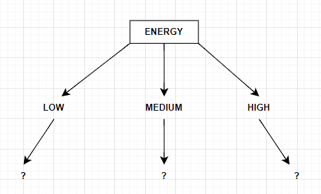
\begin{aligned} Gain (S, T) & = Entropy (S) - \sum_{v \in {M, E, A}} \frac{| S_{v} |}{| S |} Entropy (S_{v}) \\ = Entropy (S) - \frac{4}{14} Entropy (S_{T = M}) - \frac{5}{14} Entropy (S_{T = E}) - \frac{5}{14} Entropy (S_{T = A}) \\ = 0.9403 - \frac{4}{14} \times 1.0000 - \frac{5}{14} \times 0.7219 - \frac{5}{14} \times 0.9710 \\ = 0.0500 \end{aligned}

Root Node: Information Gain Attribute E¶

Attribute $E$ can take on three values (high ( $H$ ), low ( $L$ ) and medium ( $M$ )): $$ \begin{align} \ \text{Values}(E) &= H, L, M \ S_{E}&= [9_{yes},5_{no}]\ S_{E=H}&\leftarrow [5_{yes}, 0_{no}]\ S_{E=L}&\leftarrow [4_{yes}, 1_{no}]\ S_{E=M}&\leftarrow [3_{yes}, 1_{no}] \end{align} $$

The Entropy values of the three subsets of the data associated with the values of the attribute E:

$$ \begin{align*} \ \text{Entropy}(S_{E=H}) &= -\frac{5}{5} \log_2\left(\frac{5}{5}\right) - \frac{0}{5} \log_2\left(\frac{0}{5}\right) \ &= 0.0000 \ \text{Entropy}(S_{E=L}) &= -\frac{4}{5} \log_2\left(\frac{4}{5}\right) - \frac{1}{5} \log_2\left(\frac{1}{5}\right) \ &= 0.7219 \ \text{Entropy}(S_{E=M}) &= -\frac{3}{4} \log_2\left(\frac{3}{4}\right) - \frac{1}{4} \log_2\left(\frac{1}{4}\right) \ &= 0.8113 \

\end{align*} $$

Calculating the Information gain for attribute E:

\begin{aligned} Gain (S, E) & = Entropy (S) - \sum_{v \in {H, L, M}} \frac{| S_{v} |}{| S |} Entropy (S_{v}) \\ = Entropy (S) - \frac{5}{14} Entropy (S_{E = H}) - \frac{5}{14} Entropy (S_{E = L}) - \frac{4}{14} Entropy (S_{E = M}) \\ = 0.9403 - \frac{5}{14} \times 0.0000 - \frac{5}{14} \times 0.7219 - \frac{4}{14} \times 0.8113 \\ = 0.4507 \end{aligned}

Root Node: Information Gain Attribute P¶

Attribute $P$ can take on two values (yes ( $Y$ ) and no ( $N$ )): $$ \begin{align} \ \text{Values}(P) &= Y, N \ S_{P}&= [9_{yes},5_{no}]\ S_{P=Y}&\leftarrow [6_{yes}, 2_{no}]\ S_{P=N}&\leftarrow [3_{yes}, 3_{no}]\ \end{align} $$

The Entropy values of the three subsets of the data associated with the values of the attribute P:

\begin{aligned} Entropy (S_{P = Y}) & = - \frac{6}{8} \log_{2} (\frac{6}{8}) - \frac{2}{8} \log_{2} (\frac{2}{8}) \\ = 0.8113 \\ Entropy (S_{P = N}) & = - \frac{3}{6} \log_{2} (\frac{3}{6}) - \frac{3}{6} \log_{2} (\frac{3}{6}) \\ = 1.0000 \end{aligned}

Calculating the Information gain for attribute P:

\begin{aligned} Gain (S, P) & = Entropy (S) - \sum_{v \in {Y, N}} \frac{| S_{v} |}{| S |} Entropy (S_{v}) \\ = Entropy (S) - \frac{8}{14} Entropy (S_{P = Y}) - \frac{6}{14} Entropy (S_{P = N}) \\ = 0.9403 - \frac{8}{14} \times 0.8113 - \frac{6}{14} \times 1.0000 \\ = 0.0481 \end{aligned}

Root Node: Information Gain Attribute A¶

Attribute $A$ can take on two values (yes ( $Y$ ) and no ( $N$ )): $$ \begin{align} \ \text{Values}(A) &= Y, N \ S_{A}&= [9_{yes},5_{no}]\ S_{A=Y}&\leftarrow [4_{yes}, 4_{no}]\ S_{A=N}&\leftarrow [5_{yes}, 1_{no}]\ \end{align} $$

The Entropy values of the three subsets of the data associated with the values of the attribute A:

\begin{aligned} Entropy (S_{A = Y}) & = - \frac{4}{8} \log_{2} (\frac{4}{8}) - \frac{4}{8} \log_{2} (\frac{4}{8}) \\ = 1.0000 \\ Entropy (S_{A = N}) & = - \frac{5}{6} \log_{2} (\frac{5}{6}) - \frac{1}{6} \log_{2} (\frac{1}{6}) \\ = 0.6500 \end{aligned}

Calculating the Information gain for attribute A:

\begin{aligned} Gain (S, A) & = Entropy (S) - \sum_{v \in {Y, N}} \frac{| S_{v} |}{| S |} Entropy (S_{v}) \\ = Entropy (S) - \frac{8}{14} Entropy (S_{A = Y}) - \frac{6}{14} Entropy (S_{A = N}) \\ = 0.9403 - \frac{8}{14} \times 1.0000 - \frac{6}{14} \times 0.6500 \\ = 0.0903 \end{aligned}

The Information Gain for all values $$ \begin{align} \ \text{Gain}(S,T) &= 0.0500\ \text{Gain}(S,E) &= 0.4507\ \text{Gain}(S,P) &= 0.0481\ \text{Gain}(S,A) &= 0.0903\ \end{align} $$

The attribute with highest Information Gain is the attribute Energy. This will become the root node for the tree. And the decision tree after the first set of calculations becomes:

Pasted image 20240429205955.png